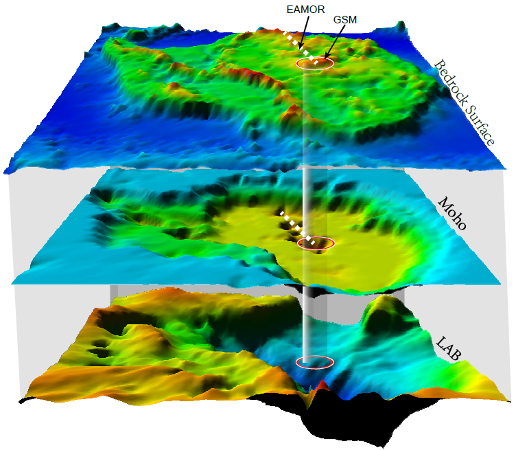
(The figure above is from An et al. [2016]. EAMOR = East Antarctic Mountain Ranges. "É amor" in portuguese = "It's love". GSM = Gamburtsev Subglacial Mountains)

Crust/Lithosphere model (AN1) of the Antarctic Plate

      Contents
1. S-velocity model (AN1-S)
2. Crustal thicknesses
3. Temperature model (AN1-T)
4. Lithospheric thicknesses (Lithsphere-asthenosphere boundary depths)
5. Curie-temperature depth Map
6. Heatflux
7. Resolution
8. References/Citations

1. Lithospheric S-velocity model (AN1-S) of the Antarctic Plate

• Compressed xyzv (lon, lat, depth, Vs) file: [download]. Each position (x/lon, y/lat) is the center of a cell. However, since the cells used in the inversion are equal-area pentagonal and hexagonal cells, the distance (in degree) between the centers of the cells varied with geographic position. Therefore, I suggest to use netCDF grid files (which can be used by Generic Mapping Tools) below.
• Compressed netCDF grid files: [download]. After uncompress it by run "tar -zxvf AN1-S_depth_grd.tar.gz", you can get 51 grid file. The name of the files are in a format: "AN1-S_hslice_${depth}.grd". If you need ascii files, you can convert them by grd2xyz (a command in Generic Mapping Tools) or other tools.

The model is paramterized into 51 layers; each layer is with a constant velocity. A depth (z) in the files is the depth of top boundary of a layer. It is noted that all depths and crustal/lithospheric thicknesses referred to here are the distance from the solid surface.

Representative horizontal slices are shown in Figure 1; transects are shown in Figure 2. They are the same as Figures 6, 7 of An et al. [2015a]. The model AN1-S is introduced in detail in An et al. [2015a].

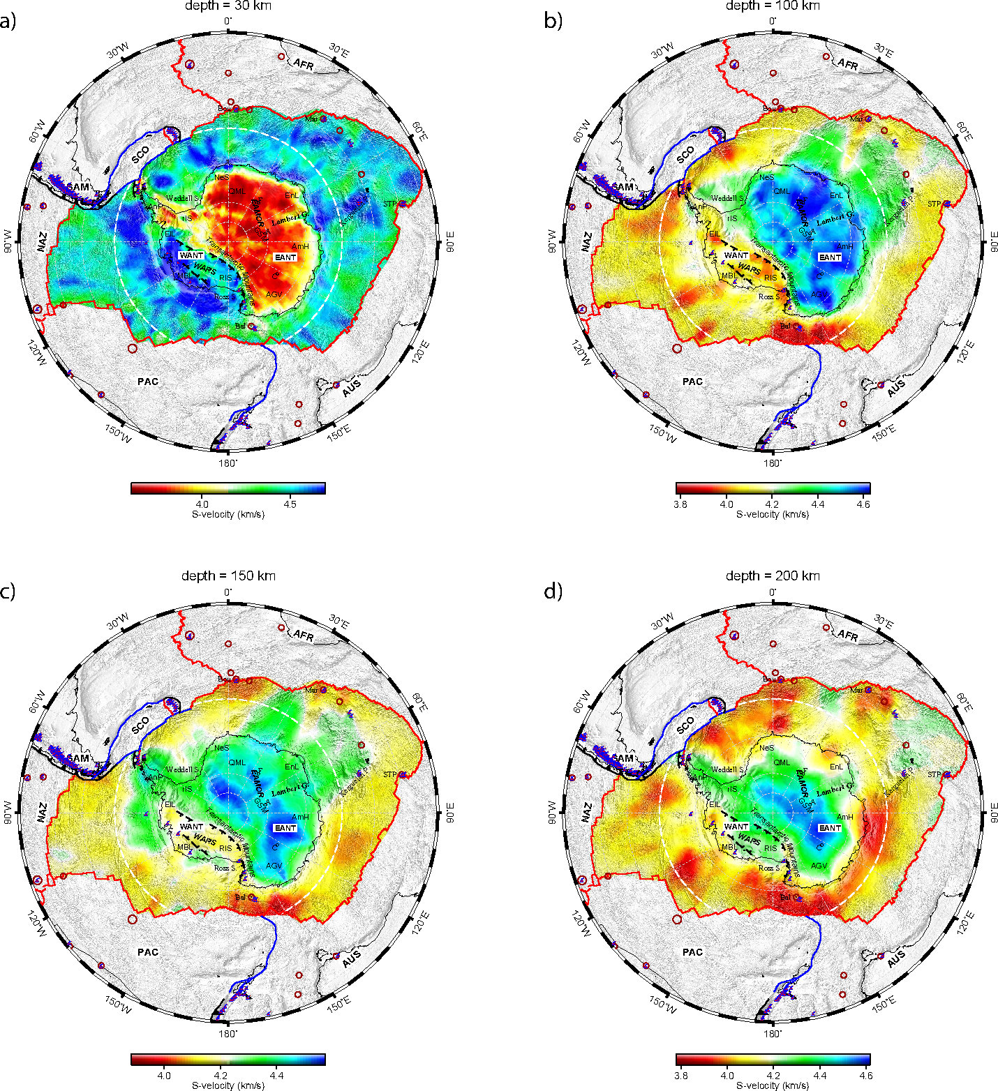
Figure 1. S-velocity maps at depths of (a) 30 km, (b) 100 km, (c) 150 km, and (d) 200 km. The figure is the same as Figure 6 of An et al. [2015a]. Download PDF.

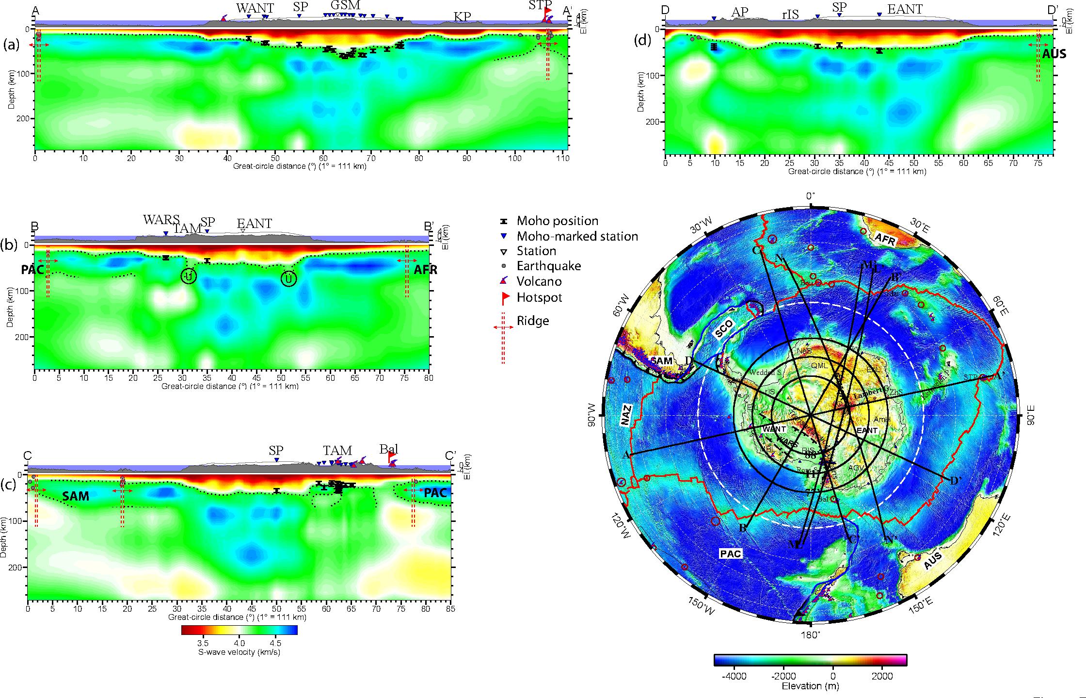
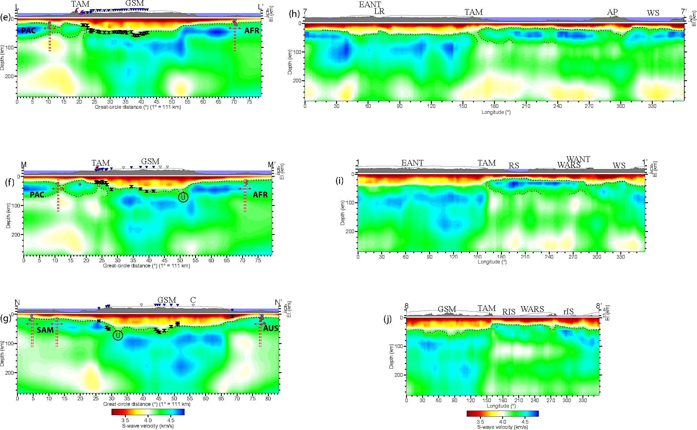
Figure 2. Representative S-velocity vertical transects of AN1-S of the Antarctic plate (=Figure 7 of An et al. [2015a]. Download PDF. All transect positions are shown in the inset plot, in which shading is the Antarctic bedrock surface from BEDMAP2 [Fretwell, et al., 2013], and in other areas is the surface topography from ETOPO2. For each transect, the black and gray shaded areas indicate continental and oceanic exaggerated topography, respectively. Black dots with error bars beneath the inverted blue-filled triangles mark the Moho positions from AN-Moho. All the inverted white-filled triangles and most of the blue-filled triangles are seismic stations used in the inversion. Earthquakes shown are from 1900 to 2007 taken from the EHB catalog [Engdahl, et al., 1998]. Black dots mark the 4.2 km/s iso-velocity contour of the inverted solution. KP = Kerguelen plateau; SP = South Pole; ZhS = Zhongshan. The others are the same or from the same sources as in Figure 1. Circles labeled with “U” mark the positions that the 4.2 km/s iso-velocity contour is too deep.

2. Crustal thicknesses / Moho depths of Antarctica

1.1. Compilation of Moho depths in Antarctica

We collected crustal thickness and/or Moho depth data from previous seismic studies (not including surface wave studies), and made a compilation of ANtarctic Moho positions (AN-Moho), under the evaluation of the quality of Moho depths. Considering that the crustal thickness or Moho depth given in previous studies may be variably defined, we corrected all thickness data to the same crustal thickness definition. Therefore, slight differences are evident between the data of our AN-Moho as compared with previous compilations and also data presented in previous studies because of different definitions.

If you need the Moho depths, please go to the page: Antarctic Moho Compilation of AN-Moho.

1.2. Moho topography

• Compressed netCDF grid file on AN1-CRUST: [download]. After uncompress it by run "tar -zxvf AN1-CRUST.tar.gz", you can get a file of AN1-CRUST.grd. If you need ascii files, you can convert it by grd2xyz.

Even though the AN1-CRUST covers the oceanic regions of the Antarctic plate, but, we note that the resolution of our model in the oceanic region is poor.

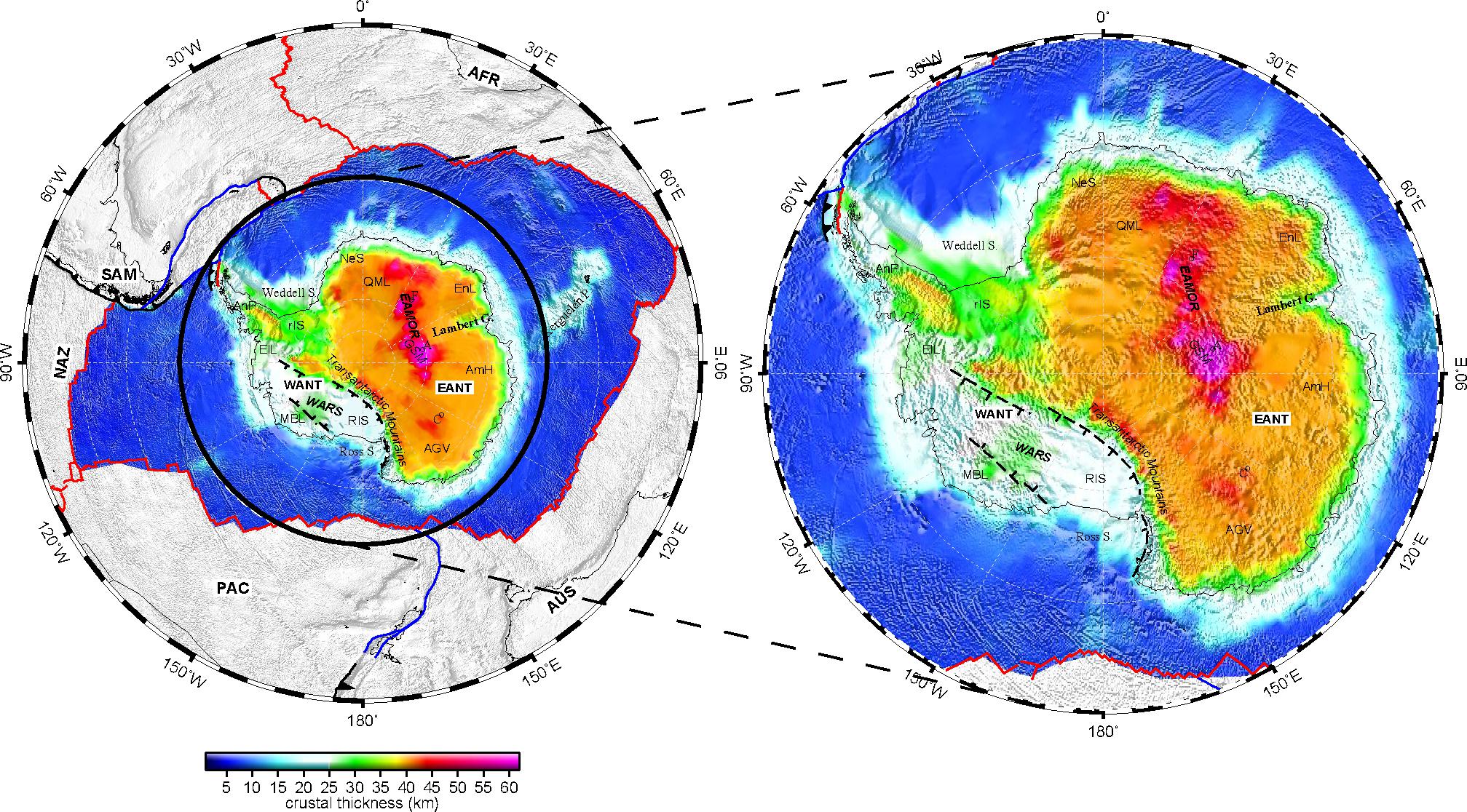
Figure 3. Crustal thickness (distance from solid (ice and rock) top to Moho discontinuity) map of the Antarctic plate [An et al., 2015a]. Download PDF.

3. Temperature model (AN1-T) of the Antarctic plate

The lithospheric temperature model (AN1-T) of the Antarctic Plate was constructed by combining the upper-mantle temperatures (Ts) of AN1-Ts converted from the above S-velocity model AN1-S, and the steady-state thermal conductive temperatures (Tc) of AN1-Tc calculated using the boundary conditions from AN1-Ts. The resolution lengths in the AN1-T model are therefore similar to those of AN1-S. Upper-mantle temperatures (AN1-Ts) is converted, following An & Shi [2006, 2007], which has its origin in the method proposed by Goes et al. [2000]. In contrast with Goes et al. [2000], An and Shi [2007] considered iron content in addition to temperature and pressure effects in the forward calculation, and used a direct grid search in the nonlinear temperature inversion. The model AN1-T is introduced in detail in An et al. [2015b].

• Compressed xyzv (lon, lat, depth, T) files: [download AN1-Ts or AN1-Tc]. Each position (x/lon, y/lat) is the center of a cell. However, since the cells used in the inversion are equal-area pentagonal and hexagonal cells, the distance (in degree) between the centers of the cells varied with geographic position. Therefore, I suggest to use netCDF grid files (which can be used by Generic Mapping Tools) below.
• Compressed netCDF grid files: [download AN1-Ts or AN1-Tc]. The name of the files are in a format: "AN1-Ts(or Tc)_hslice_${depth}.grd". If you need ascii files, you can convert them by grd2xyz (a command in Generic Mapping Tools) or other tools.

Representative horizontal slices are shown in Figures 4 & 5; transects are shown in Figure 6. They are the same as Figures 3-5 of An et al. [2015b]. The model AN1-T is introduced in detail in An et al. [2015b].

Figure 4. Upper-mantle temperature maps at depths of (a) 100 km, and (b) 150 km. The figure is the same as Figure 3 of An et al. [2015b]. Download PDF.

Figure 5. Temperature maps at depths of (a) 10 km, and (b) 20 km. The figure is the same as Figure 4 of An et al. [2015b]. Download PDF.

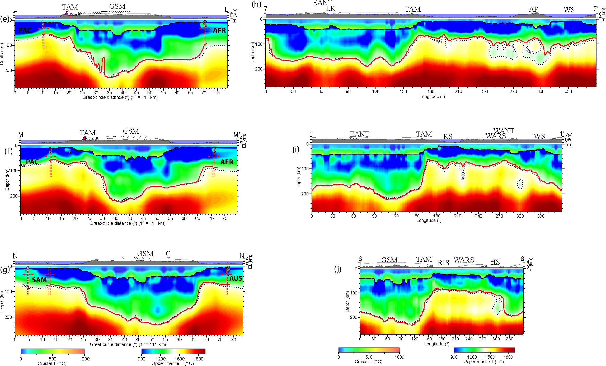
Figure 6. Representative temperature vertical transects of AN1-T of the Antarctic plate (=Figure 5 of An et al. [2015b]. Download PDF. All transect positions are shown in the inset plot, in which shading is the Antarctic bedrock surface from BEDMAP2 [Fretwell, et al., 2013], and in other areas is the surface topography from ETOPO2. For each transect, the black and gray shaded areas indicate continental and oceanic exaggerated topography, respectively. Black dots with error bars beneath the inverted blue-filled triangles mark the Moho positions from AN-Moho, red line mark the LAB position from AN1-LAB. Black dots mark the 1400 °C iso-temperature contour. KP = Kerguelen plateau; SP = South Pole; ZhS = Zhongshan. The others are the same or from the same sources as in Figure 1. The mantle temperature (right-hand color scale) was converted from the seismic velocity, and the crustal temperature (left-hand color scale) was calculated from steady-state thermal conduction. Red flags mark hotspot sites [Müller et al., 1993; Courtillot et al., 2003; Ito and van Keken, 2007] and red-filled triangles indicate volcanoes, the positions of which are from the Global Volcanism Program, Smithsonian Institution [Siebert and Simkin, 2002]. Red dashes with two arrows mark mid-ocean ridges.

4. Lithosphere-Asthenosphere Boundary depths of the Antarctic plate

• Compressed netCDF grid file on AN1-LAB: [download]. After uncompress it by run "tar -zxvf AN1-LAB.tar.gz", you can get a file of AN1-LAB.grd. If you need ascii files, you can convert it by grd2xyz.

Figure 7. Lithospheric thickness (Lithosphere-asthenosphere boundary) map of the Antarctic plate [An et al., 2015b]. Download PDF.

5. Curie-temperature depth map

Using the steady state temperatures in AN1-Tc, we generated a Curie-temperature depth map (Figure 7) with full coverage of the Antarctic Plate, assuming a Curie temperature of 580°C. All temperatures in AN1-Tc to a depth of 50 km are calculated from crustal information and from upper-mantle temperatures (AN1-Ts) at 50–95 km depth. The upper-mantle temperatures are derived from the S velocities (AN1-S) at 50-95 km depth, which are inverted from Rayleigh waves. Considering that Rayleigh waves at a period of 100 s include average S-velocity information down to ~100 km, the resolution maps at 100 s are considered the lower bound of resolution for the Curie isotherm.

• Compressed netCDF grid file: [download]. After uncompress it by run "tar -zxvf AN1-CTD.tar.gz", you can get a file of AN1-CTD.grd. If you need ascii files, you can convert it by grd2xyz.

Figure 8. Map of the Curie temperature (580°C isotherm) depth of the Antarctic plate [An et al., 2015b]. Download PDF.

6. Heatflux

During calculating crustal temperatures of AN1-Tc An et al. [2015b], we also obtained the surface heat flux in Antarctica. Similar to Curie isotherms, the resolution maps at 100 s are considered the lower resolution bounds of heat flux results.

• Compressed netCDF grid file: [download]. After uncompress it by run "tar -zxvf AN1-HF.tar.gz", you can get a file of AN1-HF.grd. If you need ascii files, you can convert it by grd2xyz.

Figure 9. Map of heat flow in Antarctica [An et al., 2015b]. Download PDF.

7. Resolution lengths of AN1

• Compressed netCDF grid file: [download]. After uncompress it by run "tar -zxvf hresolution.grd.tar.gz", you can get three resolution grid files. If you need ascii files, you can convert it by grd2xyz.

The lateral resolution maps are of Rayleigh waves and can represent the lateral resolution of AN1-S.

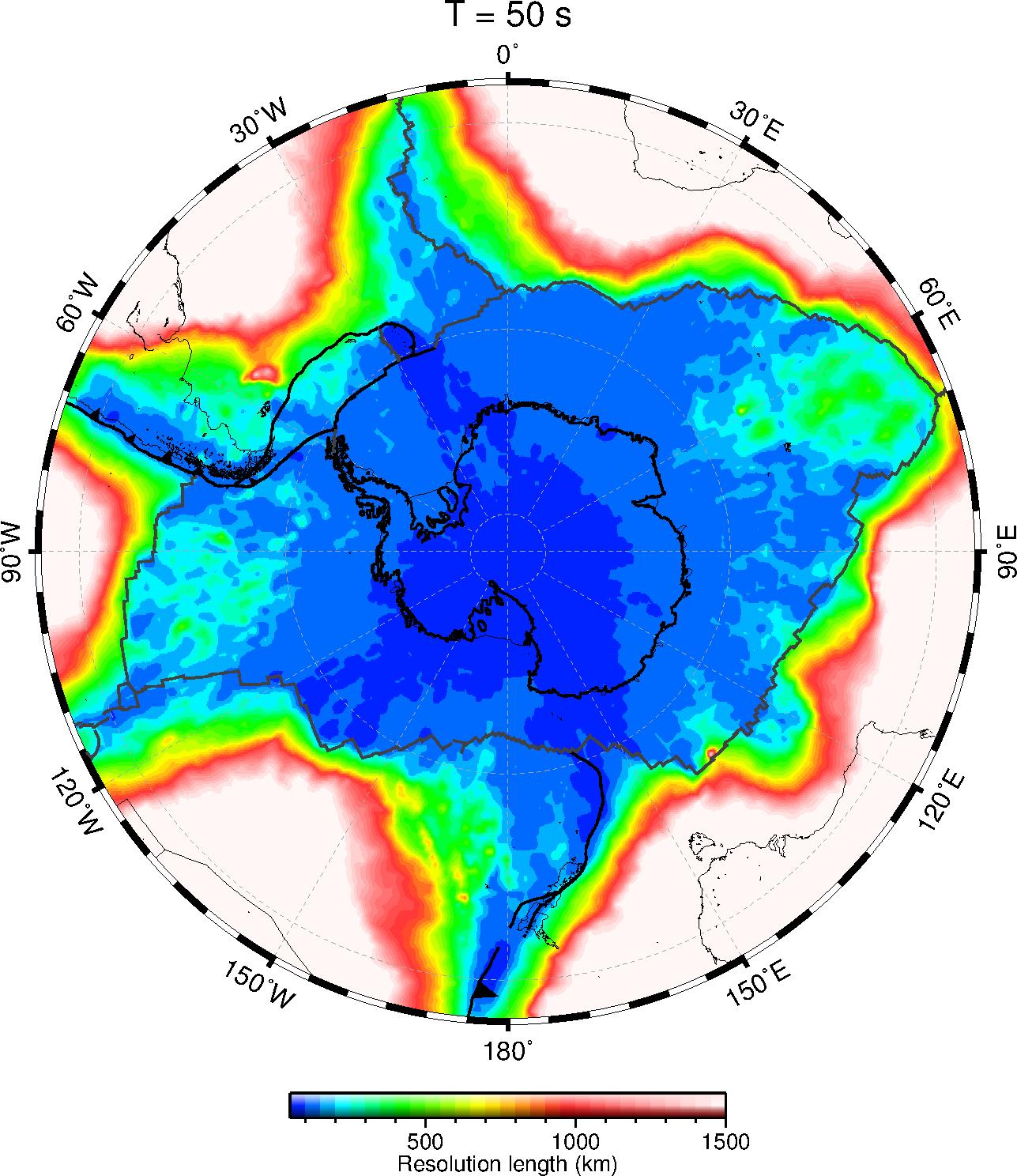
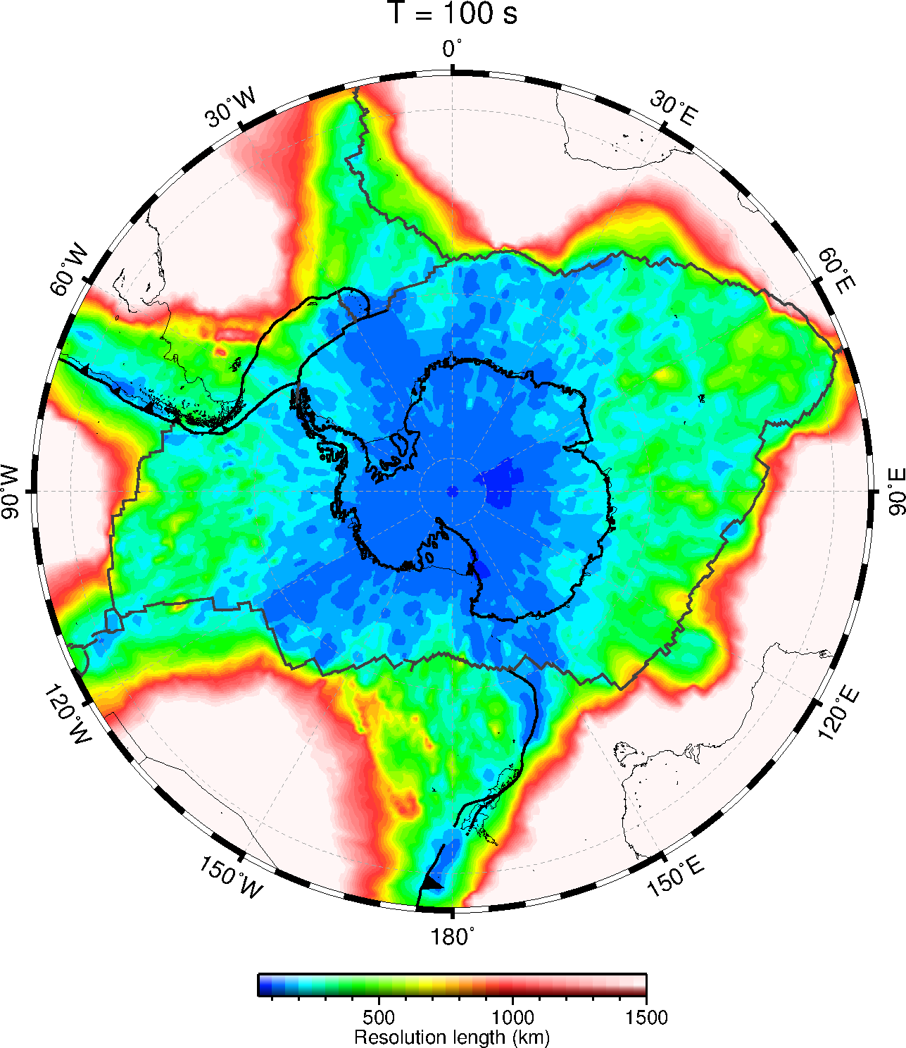
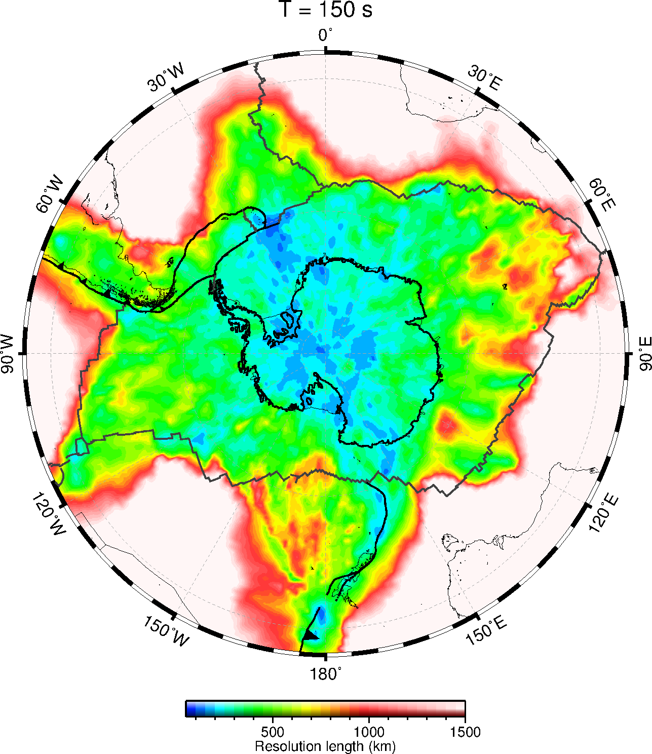
Figure 10. Resolution lengthes for Rayleigh wave dispersions at three periods [An et al., 2015a]. Download PDFs.

8. References:

An Meijian, Douglas Wiens, Zhao Yue, 2016, A frozen collision belt beneath ice: an overview of seismic studies around the Gamburtsev Subglacial Mountains, East Antarctica. Advances in Polar Science, 27(2): 78-89. doi:10.13679/j.advps.2016.2.00078. [Full Text ] [PDF].

An Meijian, Douglas Wiens, Zhao Yue, Feng Mei, Andrew A. Nyblade, Masaki Kanao, Li Yuansheng, Alessia Maggi, Jean-Jacques Lévêque, 2015a, S-velocity Model and Inferred Moho Topography beneath the Antarctic Plate from Rayleigh Waves. J. Geophys. Res., 120(1),359–383, doi:10.1002/2014JB011332 [Full text]. [PDF]. [Merged supporting file].

An Meijian, Douglas Wiens, Zhao Yue, Feng Mei, Andrew A. Nyblade, Masaki Kanao, Li Yuansheng, Alessia Maggi, Jean-Jacques Lévêque, 2015b, Temperature, lithosphere–asthenosphere boundary, and heat flux beneath the Antarctic Plate inferred from seismic velocities, J. Geophys. Res., 120(12), 8720–8742, doi:10.1002/2015JB011917 [Full text]. [PDF]. [Supporting file].

Feng Mei, An Meijian, 2010, Lithospheric structure of the Chinese mainland determined from joint inversion of regional and teleseismic Rayleigh-wave group velocities.  J. Geophys. Res., 115, B06317, doi:10.1029/2008JB005787. [Full text] [PDF]

An Meijian and Shi Yaolin, 2007, Crustal and Upper-mantle Temperature of the Chinese Continent.  Sci China (Ser. D), 50(10), 1441-1451, doi:10.1007/s11430-007-0071-3. [Full text] [PDF]

An Meijian and Shi Yaolin, 2006, Lithospheric Thickness of the Chinese Continent.  Phys. Earth Planet. Ints., 159, 257-266, doi:10.1016/j.pepi.2006.08.002. [Full text] [PDF]