PROBLEM: In an inversion using both reference model and higher-order Tikhonov regularizations, e.g., flatness (or called differential smooth) or smoothness, bad discontinuity in the refenrence model is expected to be corrected, but the correction is difficult because of the regularizations. The regularizations tend to minimize the variations in the inverted model perturbations, i.e., to prevent the correction.

SOLUTION: A viable approach to overcome this shortcoming is to adapt the regularization for the reference model such that a sharp variation around a given position in the reference model (regardless of whether the variation is true or false) receives a smaller weighting in the regularizations (An, 2020, doi:10.1007/s00024-020-02530-z). For example, set the weight in a form:

EXAMPLE: Here is an example of a linearized inversion of surface wave dispersion by surf96 (code of Herrmann's Computer Programs in Seismology). In surf96, differential smooth (regularization) matrix is defined as:

Figure below shows results using two different starting models. In the tests, all red models resulted by An (2020)'s differential smoothness are better (closer to true model) than blue models by general differential smoothness. The initial reference model B is with bad discontinuity, which is hard to be corrected by a general differential smooth (in blue model), but is easily by the new adaptive smooth (in red model).

	Using initial reference model A	Using initial reference model B
Result at iteration 5: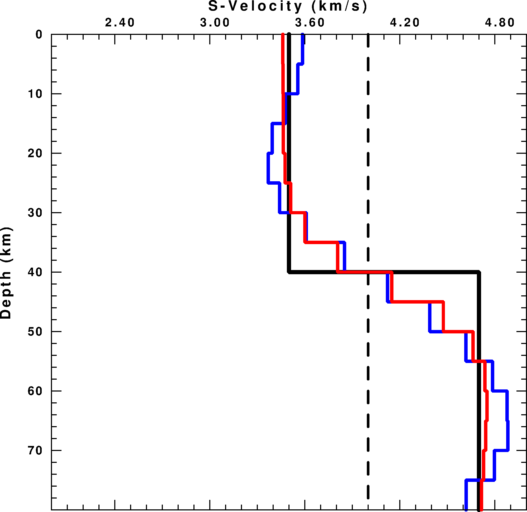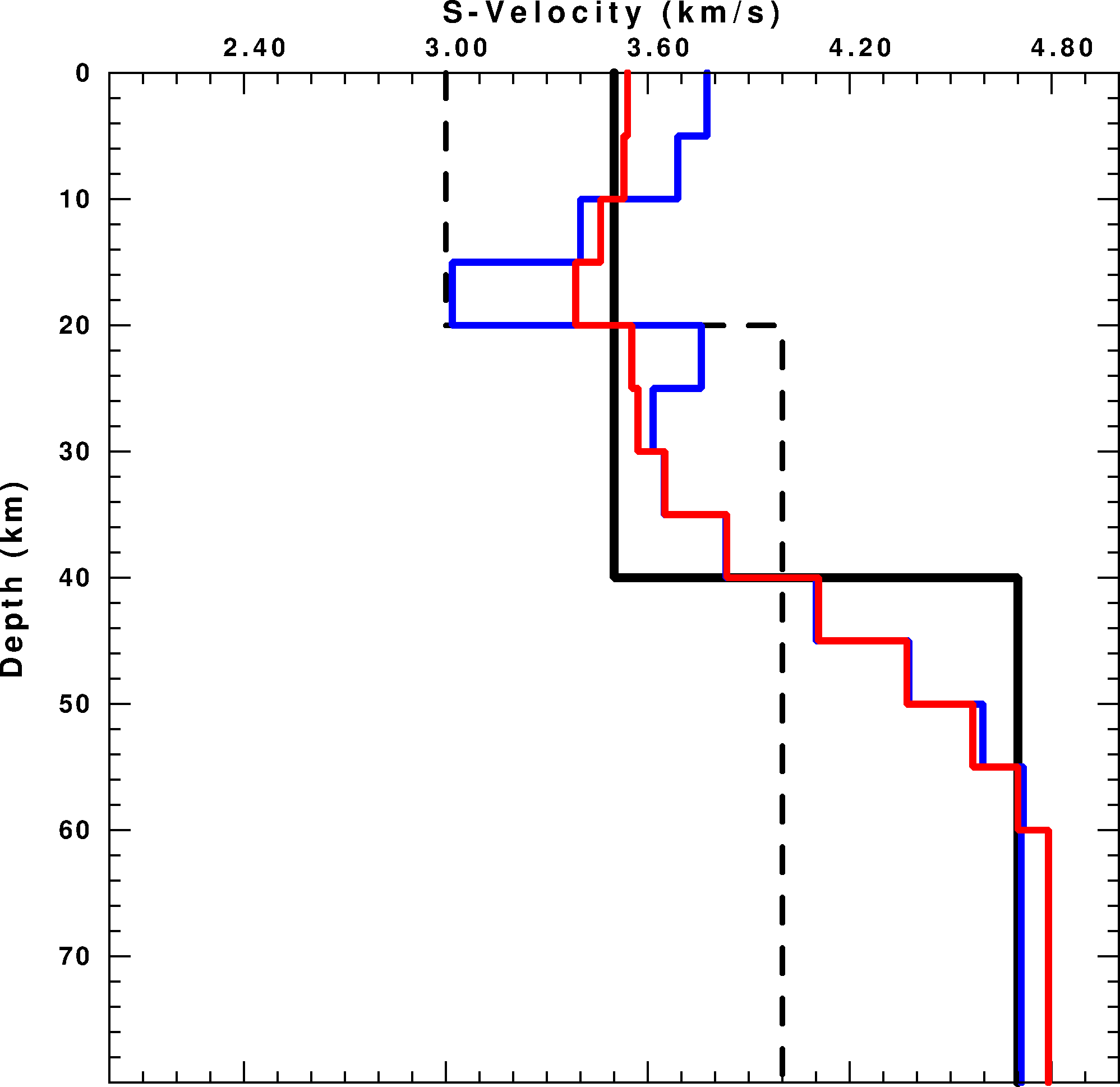
Result at iteration 100: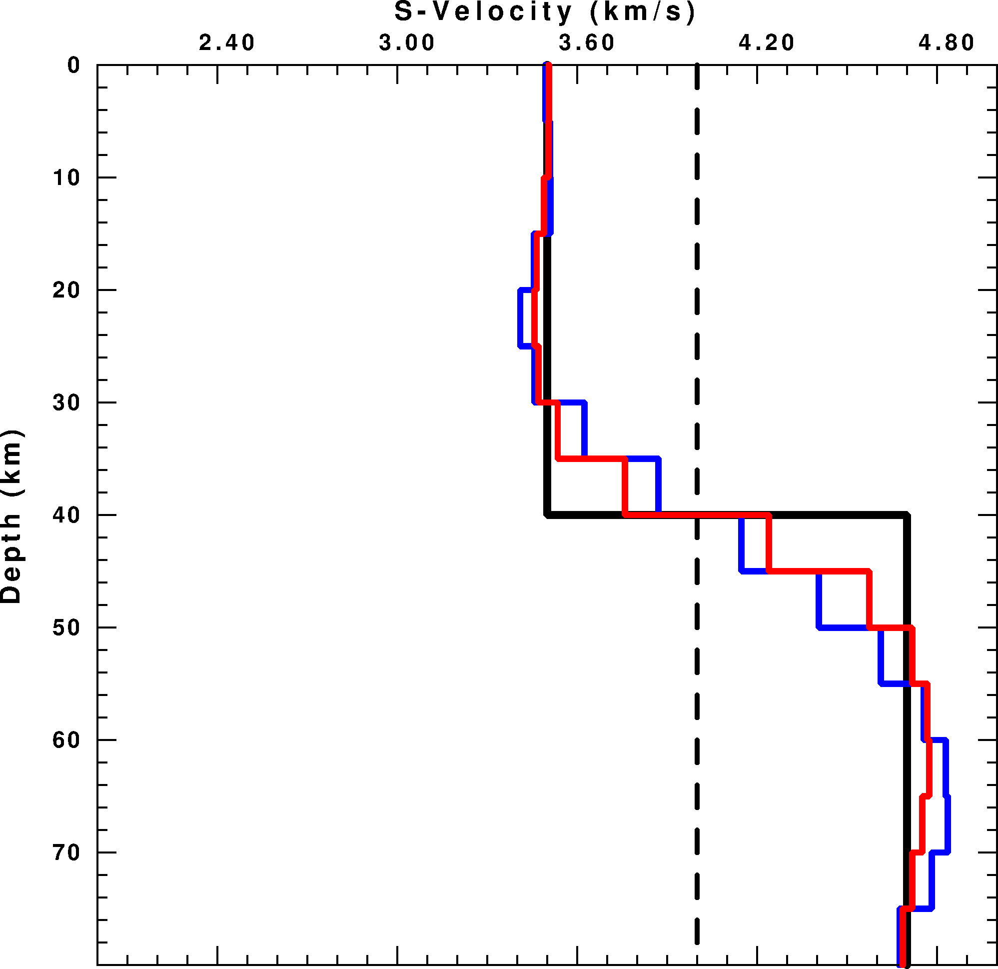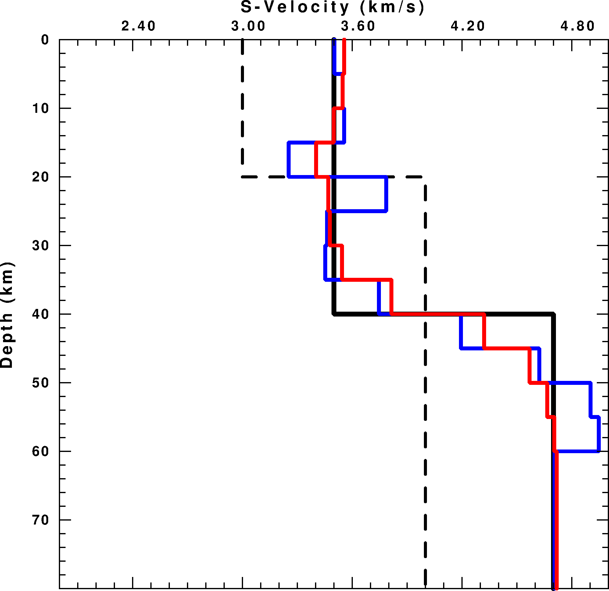
Figure 1. Synthetic test results. Blue line is resulted by surf96 with option 36 1.

The above reference model-based regularization adaptation is explained in An (2020, PAAG) (go to paper pdf ...)

get_statistical_resolution_length V1.3, updated on 08/10/2014. The program directly inverts for statistical resolution lengths/matrix from synthetic models and their respective solutions. The package includes examples, which are the same as in An (2012). You can download the codes and examples by click [here]. The codes in V1.3 can calculate resolution lengths for specific parameter IDs, which is useful for an inversion with many parameters, e.g., to obtain resolution lengths for the parameters just along a trasect for a 3D-model inversion. The change in V1.3 is fix a bug in V1.2 when the number of parameters is <50. The changes made in V1.1 than V1.0 is to improve computation efficiency and use less memory.

The resolution matrix of an inverse problem defines a linear relationship in which each solution parameter is derived from the weighted averages of nearby true-model parameters, and the resolution matrix elements are the weights. Resolution matrices are not only widely used to measure the solution obtainability or the inversion perfectness from the data based on the degree to which the matrix approximates the identity matrix, but also to extract spatial resolution or resolution length information.

Resolution matrices presented in previous spatial-resolution analysis studies can be divided into three classes: direct resolution matrix, regularized/stabilized resolution matrix, and hybrid resolution matrix. The direct resolution matrix can yield resolution length information only for ill-posed inverse problems. The regularized resolution matrix cannot give any spatial-resolution information. The hybrid resolution matrix can provide resolution length information; however, this depends on the regularization contribution to the inversion. The computation of the matrices needs matrix operation, however, and this is often a difficult problem for very large inverse problems.

Here, a new class of resolution matrices, generated using a Gaussian approximation (called the statistical resolution matrices), is proposed whereby the direct determination of the matrix is accomplished via a simple one-parameter nonlinear inversion performed based on limited pairs of random synthetic models and their inverse solutions. Tests showed that a statistical resolution matrix could not only measure the resolution obtainable from the data, but also provided reasonable spatial/temporal resolution or resolution length information. The estimates were restricted to forward/inversion processes and were independent of the degree of inverse skill used in the solution inversion; therefore, the original inversion codes did not need to be modified. The absence of a requirement for matrix operations during the estimation process indicated that this approach is particularly suitable for very large linear/linearized inverse problems. The estimation of statistical resolution matrices is useful for both direction-dependent and direction-independent resolution estimations. Interestingly, even a random synthetic input model without specific checkers provided an inverse output solution that yielded a checkerboard pattern that gave not only indicative resolution length information but also information on the direction dependence of the resolution.

The method is explained in my paper of An (2012, GJI) (go to paper pdf ...)

    sac2local * ../*

GetEvts V2.5, released on 20/02/2004, slices events to sac format from data in MSeed, SEGY, SACs, etc. GetList V2.0, released on 20/02/2004, transforms QED_daily to earthquake list which is used by GetEvts. These programs are made for seismological laboratory, IAG-USP. Downloadable bins for Win, Linux or Unix. This downloadable package includes two example shells (getlist1.sh and getlist2.sh) explaining how to use getlist.

Getevts uses: the event list outputted from getlist; a file includes the information of stations; original data.

Help of getlist can be shown by running it "getlist". Below is the information of columns ($n) in the output file by getlist:

Record begin time:

$1 -- year

$2 -- year day (or jday)

$3 -- hour

$4 -- minute

$5 -- second

$6 -- record length (minute)

Event magnitude:

$7 -- mb

$8 -- Ms

Event time:

$9 -- year

$10 -- year day

$11 -- hour

$12 -- minute

$13 -- second

Event position:

$14 -- latitude

$15 -- longitude

$16 -- depth

Event-station relation:

$17 -- Az

$18 -- Baz

$19 -- Dist

$20 -- Gcarc